The fourth part of the article "Method of load currents calculation"
It is not a surprise, but we will talk not about overhead power transmission lines, but about extended underground utility systems. It can be, for example, metal conduits or simply very long grounding buses. The running inductance of such utility system is approximately the same as of the overhead power transmission line. The capacity per unit length doesn't increase significantly (relative dielectric permeability of soil ε, as a rule is not greater than 10) and that is why, the condensance leakage current in many situations is much less than the current in the grounding devices. But the conductive running cross conduction, determining the lightning current leakage through the surface of the utility system contact with the ground is very significant. As known, the ground resistance of a grounding bus with the radius r0 and length l, laid in the ground with electrical resistivity ρ at the depth h, is equal to

(17)
For example at a lenth 200 m and radius of 5 m, a metal pipe in the ground with ρ =100 Ohm at the laying depth of 1 m will have the ground resistance of 1 Ohm. It is comparable not only with the ground resistance of the protected object, but even with a typical ground resistance of electric substation. It is clear that such a significant parameter should be considered in the calculation.
Now we should remember how the transition process from the equivalent network with distributed parameters to the focused scheme was carried out. In fact, instead of a great number of short potential cuts, there was the only one, the length of which was equal to the length of the utility system, and inductance - its complete inductance. The role of inductance did not change a lot. Like in the distributed network, it divides the grounding resistances on the ends of the utility system. As concerns the capacity of the utility system, it was neglected, because the leakage current through the container was neglectively small compared to the current through grounding resistance. For an underground cable, like it has just been shown, the conductive leakage is more crucial than the capacity one. Thanks to it, the utility network may have a very low grounding resistance. Of course, we can try to display it with additional resistors, placed in parallel at the ends of the utility system, as shown in fig. 11. But since the resistors Rg are comparable with the grounding resistances R1 and R2, the mode of the current distribution will be very corrupted. The calculated data can serve as an illustration, see fig.12.
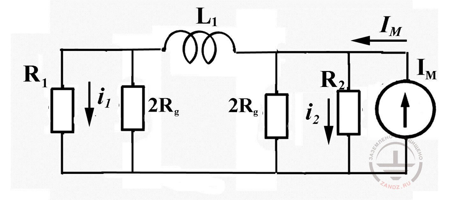
Fig. 11. To the justification of the equivalent circuit of underground utility system in conductive ground
They were obtained by the calculation on the circuit with the concentrated parameters (fig. 11) for a pipeline 200 m in length and 5 cm in radius. It was supposed, that it was placed in the ground with a resistivity of 100 ohm m at the depth of 0.5 m. The grounding resistance of an object, hit by a lightning, is taken equal to 10 Ohm, the resistance on the other end of the pipleline - 1 Ohm. For comparison in Fig. 12 you can see the calculated values of currents, obtained in the equivalent circuit with distribution parameters. There is not much in common between them. It is clear, that we cannot avoid a strict calculation.
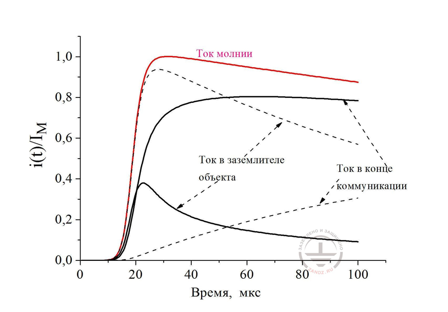
Fig. 12. The comparison of the calculation results of the lightning current distribution in the presence of an underground pipeline 200 m long between the concentrated ground electrodes in the equivalent circuit with distributed (solid curves) and lumped parameters (dashed curves)
Ток молнии – lightning current
Ток в заземлителе объекта- current in the object ground electrode system
Ток в конце коммуникации – current in the end of utility
Время, мкс – time, ms
In major part of practical situations, when it is possible to neglect the capacity current leakage in comparison to the conductive leakage, the system of equations in differential derivatives looks like


(18)
and repeated differentiation on x is reduced to a known diffusion equation

(19)
Here G is a running conductivity of the leakage to the ground, and running resistance of underground utility system R is excluded from the equations due to its nullity. The algorithm of the numerical solution of equation (19) does not differ from the one studied in section 3 for a plot of an overhead transmission line. But in this case, it is more convenient to determine the currents in lateral cuts of the utility system by a direct sweep and then calculate the strain of the cuts by a reverse sweep.
Difference expression is used for a direct sweep
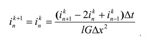
(20)
At that, the current on the final N-cut of the utility communication, connected with the ground electrode Rk, is counted by the following expression

(21)
and the current in the first cut is expressed through the lightning current IМ and the grounding resistance of the start of the utility system Rn

(22)
Reverse pass, necessary for the calculation of voltage, except uses the expression

uses the expression

(23)

(24)
This is thThe algorithm of a computer calculation is not principally different from the one, that was formed for an overhead power line in section 3.
Initially, it is necessary to know the sizes of underground utility system and calculate the grounding resistance at the direct current Rg according to formula (17). It is necessary in order to determine the running conductivity of the leakage G =1/ (lRg). Lengh and radius of the utility system are also necessary for the calculation of its running inductance (see formula (26) from the next section). Grounding resistances on the ends of the utility system will be required as source data.
Then, the following operations are carried out:
The calculation cycle is repeated for a certain time moment, increasing with a pitch ∆t up to the ultimate set.
Exact solution shown in Fig.12, is carried out according to this algorithm. It is useful to notice, that it is applicable at any values of grounding resistance on the ends of the utility system. If to put them very large, for instance 106 Ohm, the mode of lightning current leakage from the utility systems will be defined only by its own conductivity. Then, we can get the time change dynamics of the grounding resistance of an extended grounding bus by dividing the voltage in the beginning of the utility system (cut № 1). This parameter is also crucial for calculation of lightning overvltage.
In conclusion, we would like to note, that the algorithm fits the calculation at any form of lightning current pulse. For that, it is enough to introduce a corresponding analytical expression for IМ(t) into the calculation instead of formula (9). For instance, calculated data in fig. 13 characterize the dynamics of grounding resistance change in time for a horizontal conductor with the parameters, similar to the used ones for fig. 12. It was suppposed, that the specific soil resistance was equal to 100 Ohm *m and the lightning current pulse changes in time according to the biexponential rule

(25)
with time constants a = 0,8 ms-1 and b = 0,007 ms-1 (approximately corresponds to the typical current pulse of the first component of lightning with a front of ~ 5 ms and duration ~ 100 ms).
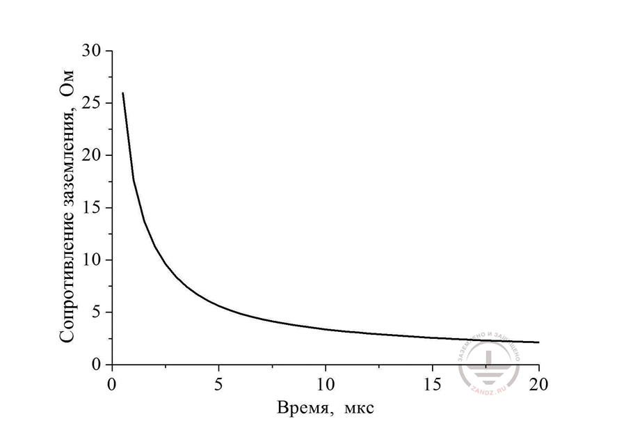
Fig. 13. The dynamics of changes in time of the horizontal pipeline ground resistance of 200 m long and 5 cm in radius, put in the soil with ground resistivity ρ = 100 Ohm m at the depth of 0.5 m
Сопротивление заземления, Ом – ground resistance, Ohm
Время, мкс – time, ms
Loss of time for the calculation was not useless, - we can see that during the first 10 ms, conductor's grounding resistance was reduced by an order of magnitude.
E. M. Bazelyan, DEA, professor
Energy Institute named after G.M. Krzyzanowski, Moscow
Read more "5. Useful recommended practices on the calculation of SPD load currents"
See also:
- Video recording and transcript of the webinar with Prof. E.M. Bazelyan "Why do we need SPDs"
- Principles of choosing surge arresters in low-voltage electric networks on the example of Leutron devices
- Free webinars for designers of grounding and lightning protection
- Grounding and lightning protection projects in dwg, pdf formats
- Free consultations and assistance in calculation of grounding and lightning protection
Related Articles:
 Lightning Protection of Large Territories: Parks, Grounds, Plant Territories. Page 1
 Lightning Protection of Large Territories: Parks, Grounds, Plant Territories. Page 2
 Lightning Protection of Large Territories: Parks, Grounds, Plant Territories. Page 3