The fifth part of the article "Methodics of calculation of SPD load currents"
The inductivity of overhead line cut with the length l at the average height of its wires suspension in the passing h can be determined according to the calculated formula

[mcH], (26)
where all geometric sizes are entered in meters and the following value is used as an effective radius of n-wire line

(27)
Here r - radius of metal wires, d - average distance between the wires. It is useful to note, that no special accuracy in determination of the radius is required, because the inductivity of the wire weakly depends on it, logarithmically.
The time interval for the calculation is chosen the way to provide the drawing of the lightning current pulse front. For example, at the front time of 10 ms (pulse 10/350 ms, on which SPD of the I protection level are chosen), gives quite a satisfactory result with the interval of 1 ms, at which the front is being drawn by 10 calculation points; at an interval of 0,1 ms (100 calculated points on the front) the result of the calculation appears to be brilliant. The question about the current pulses of the next components appears immediately. As a rule, their current is not counted at the choice of SPD, but the estimation of its distribution over the separate metal structures of the object can appear to be important (for example, at the calculation of EMF of density inside the protected obejct). In order to transfer the current pulse front of the next component with the ultimate duration of 0,25 ms, it is necessary to reduce the time interval of the calculation up to 0,02 - 0,01 ms. For a modern computer, this is not a problem even in case when the full calculated time is counted by hundreds of microseconds. If, for some reason, the volume of the calculation should be reduced, it is possible to hold two consequitive calculations - first with the indicated small calculation pitch to the time of 0,5 - 1,0 ms and the next with the calculation pitch 10-100 times more to the maximally required time moment. The obtained results are easy to bring to a common function connection.
If there is a problem with a computer - the situation cannot be considered fatal at a working scientific calculator. It is necessary to calculate lightning current values with a quite unfortunate formula (9). Everything else can be made manually.
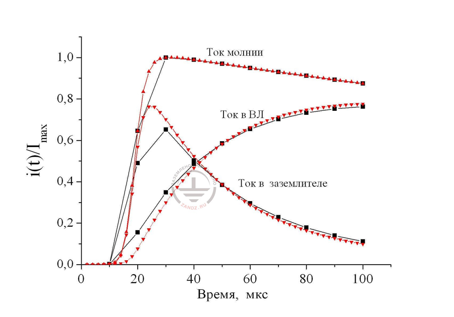
Fig. 14. To the estimation of possibilities of manual calculation of lightning current in the object utilities
Ток молнии – lightning current
Ток в ВЛ – current in overhead power transmission line
Ток в заземлителе – current in the ground electrode system
Время, мкс – time, ms
The matter is in the exclusive resistance of the numerical solution of the studied equations. In the calculations, it is possible to bring the time pitch without large fault to 1-2 ms, when it is necessary to reproduce lightning current pulse front and then operate with the pitch of about 10 ms. On fig. 14 you see the result of such calculations for the conditions, similar to the ones presented on fig. 5. The red designations on the charts refer to the calculation with the time pitch of 2 ms, black - 10 ms, all the calculated points are marked. If not to spend time to the reproduction of the first 10 ms with an almost null current (the contrary flexure of the EIC standard compliers'), the lightning current pulse front and the currents in the utilities corresponding to it, can be quite described by 10 calculated points. At that, it is necessary to start the calculation not with t = 0, but with t = 10 ms. 10 more points with the pitch of 10 ms reproduce the dynamics of currents' change in the next 100 ms on the pulse tail. In total, there are 20 calculated pitches. It is available even to a not very patient engineer with a calculator in hands.
Can we do it even simpler? Yes, but with some loss of accuracy. For that, it is necessary to remember about the three parameters of the transit process: high voltage transmission line inductivity and grounding resistance at its ends. Lightning current is initially limited by the high voltage transmission line inductivity and only then goes to the object ground electrode system. Its penetration into the line happens with the time constant

(28)
In the set mode (at t>>T) the current is distributed in reverse proportion to the grounding resistance values
; (29)
Considering everything said above, it is enough to build the lightning current pulse of the singular amplitude according to formula (9) in order to estimate the currents (better using a drawing machine, but can be done point by point). And then, build the function chart by displacing the vertical axis to about 10 ms in order to skip the almost null values.

(30)
as it was done in fig.15. The starting part of the curve, describing current i1(t) from point 1 to point 2 can be considered coinciding with the lightning current, and from point 2 to point 3 and further - with the function built f(t). Deviation from the results of the precise
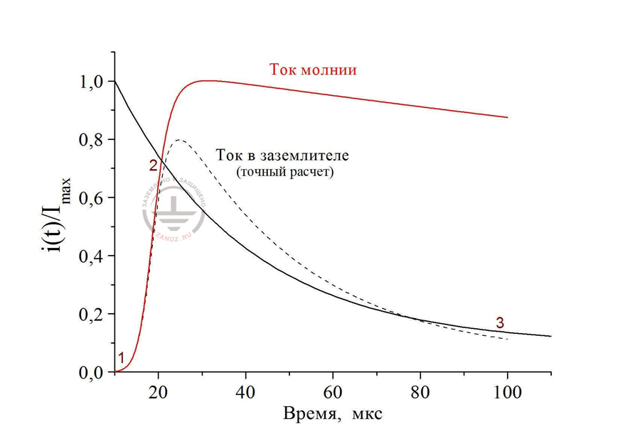
Fig. 15. To the approximate estimation of current in the object utilities
Ток молнии – lightning current
Ток в заземлителе (точный расчет) – current in the ground electrode system (precise calculation)
Время, мкс – time, ms
calculation lies within 15%. The high-voltage transmission line current i2(t) is again determined as the difference obetween the lightning current and the found current i1(t).
In the conclusion it is better to note, that the primitive estimation of current distribution with a graphical method, which was given above, gives a good result at the lightning strike into the overhead power line, feeding the protected object. For this purpose, the time constant of the process should be defined through the sum of inductivity of overhead power transmission line parts from the strike point
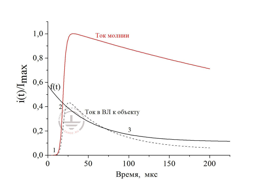
Fig. 16. The quantitative estimation of currents distribution at the lightning strike into the middle of the overhead power transmission line part
Ток молнии – lightning current
Ток в ВЛ к объекту – current in overhead power transmission line to the object
Время, мкс – time, ms
lightning to the object and to the substation feeding it

(31)
and present the exponential function in the form

(32)
The results of the estimations can be seen in fig. 16, which is completely similar with its structure to fig. 15. As before, the current, branching along the over-head power transmission line in the direction of a substation, is defined as
i2(t)=IМ(t)-i1(t)
With you luck!
E. M. Bazelyan, DEA, professor
Energy Institute named after G.M. Krzyzanowski, Moscow
See also:
- SPD selection guide
- Principles of choosing surge arresters in low-voltage electric networks on the example of Leutron devices
- Free webinars for designers of grounding and lightning protection
- Grounding and lightning protection projects in dwg, pdf formats
- Free consultations and assistance in calculation of grounding and lightning protection
Related Articles:
 Lightning Protection of Large Territories: Parks, Grounds, Plant Territories. Page 1
 Lightning Protection of Large Territories: Parks, Grounds, Plant Territories. Page 2
 Lightning Protection of Large Territories: Parks, Grounds, Plant Territories. Page 3